1. Deep Learing with Colab (an introduction)
This tutorial demonstrates training a simple Convolutional Neural Network (CNN) to classify MNIST Dataset.
1.1. CNN in a glance
The Convolutional Neural Network (CNN) is a class of Deep Learning Netower extensively used in image analysis (Computer Vision). The main feature is the Convolution Layer, which replaces the classic Perceptron (i.e., the “Neuron” of a Neural Network) with a “Filter” containing the “weights” that convolute the input from the previous layer Fig. 1.7.
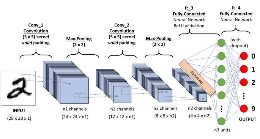
Fig. 1.7 Example of CNN architecture to classify handwritten digits.
Let see some possible layer that you can use in a CNN:
1.1.1. Convolution layer
Fig. 1.8 Convolutional layers example with differnt stride and padding hyperparameters.
The convolutional layer is the Neural Networks (NN) solution to replace the fully connected Perceptron layer.
When dealing with n-dimensional tensor (with n > 1), the memory required to build a classic NN raises fast and reaches a value that makes
the use of this technique unuseful. The solution is, instead to connect each neuron to every input pixel, we use a filter (a.k.a. kernel)
which scans the previous layer’s input, and the resulting product (convolution) builds the output.
The main and crucial hyperparameter of this layer is the stride and padding, Fig. 1.8:
Stride is the number of pixels shifts over the input matrix.
When the stride is 1 then we move filters to 1 pixel at a time.
When the stride is 2, then we move the filters to 2 pixels at a time and so on.
Padding is the amount of zeoro-element added to an image (input tensor) when it is being processed by the kernel of a CNN.
Changin the stride and padding chenge the output layer shape, and the output width or height can be compute with the
(1.1)
where \(O\) is the output width/height, \(I\) is the input width/height, \(K\) is the kernel size, \(P\) is teh padding and \(S\) is the stide.
Note with a kernel of 3x3 (\(K=3\)) we have that settintg the stride=None and padding=2 the input and output layer
have the same size (this is usualy called “same” padding).
1.2. Colab
Colab is a free Jupyter notebook environment that runs entirely in the cloud. Here we can use all the libraries available for python, and for working with the Neural network, we have a lot of them. To name some: scikit-learn, pyThorch and Tensorflow.
In this tutorial, we are going to use the latter one: Tensorflow (TF).
Let’s go to Colab https://colab.research.google.com/ open an account and a new notebook.
It is a Jupyter notebook; therefore, we can write and run the blocks element. These can be a code block or a text block, Fig. 1.10.
In the first one, we can write everything is python readable, in the second everything si Markdown
readable. To run the block, we can click on the “play” button on the side or use the shortcut shift+enter.

Fig. 1.10 Coolab blocks view.
Before to everything, we have to set up the cloud driver, go to the “runtime” drop-down menu, select “change runtime type” and choose TPU in the hardware accelerator drop-down menu (Fig. 1.11). (TPU stand for Tensor Processing Unit (TPU) is an AI accelerator application-specific integrated circuit (ASIC) developed by Google)

Fig. 1.11 Change runtime type popup.
1.3. Handwritten number recognition with CNN
To build a NN, we go throw the following steps:
Environment set-up.
Data collection and preprocessing.
Model building.
Model compiling (loss function, training strategy)
Training.
Validation.
For this tutorial, we are going to build a CNN to recognize the handwritten number present in the database MNIST. If you want to use the top in the market go to see the last model winner of the famous Image-Net challenge
1.3.1. Environment set-up
First of all let’s open a section by createing a new Text block and writing inside the code:
# Libraries
Then we load all the python libraries needed for this project.
In [1]: %tensorflow_version 2.x             # We want use TF version >= 2.0
   ...: import tensorflow as tf             # The NN backend
   ...: from tensorflow.python.keras import layers, Sequential, Model, regularizers
   ...: import matplotlib.pyplot as plt     # To plot
   ...: import numpy as np                  # To work with arrays
   ...: import random
   ...: from tqdm import tqdm               # To show progressive bar
We check if the TPU is working.
In [2]: # Check that we are using a TPU
   ...: try:
   ...:     tpu = tf.distribute.cluster_resolver.TPUClusterResolver()  # TPU detection
   ...:     print('Running on TPU ', tpu.cluster_spec().as_dict()['worker'])
   ...: except ValueError:
   ...:     raise BaseException('ERROR: Not connected to a TPU runtime; please swithc runtimes  Runtime > Change Runtime Type > TPU!')

Running on TPU  ['10.115.241.50:8470']
1.3.2. Data collection and preprocessing
In this part we downolad and look at out dataset. The MNIST (Modified database National Institute of Standards and Technology) is a collection of 70.000 handwritten 10-digit images, downsampled in size (28 × 28 pixels), in black and white and therefore with only one color channel.
First, we open a new section of our Notebook.
# Data collection and preprocessing
Then we load the database. Because it is a standard database (a sort of Hello World for CNN), it is already included in TF, so we only need to run the following function:
In [3]: mnist = tf.keras.datasets.mnist
   ...: (train_images, train_labels), (test_images, test_labels) = mnist.load_data()

Downloading data from https://storage.googleapis.com/tensorflow/tf-keras-datasets/mnist.npz
11493376/11490434 [==============================] - 0s 0us/step
Let’s look how many images we have:
In [4]: print(f"Train Images:{train_images.shape}")
   ...: print(f"Train Labels:{len(train_labels)}")
   ...: print(f"Test Images:{test_images.shape}")
   ...: print(f"Test Labels:{len(test_labels)}")

Train Images:(60000, 28, 28)
Train Labels:60000
Test Images:(10000, 28, 28)
Test Labels:10000
Thus we have 60k images for the training and 10k for the test (86%-14% split).
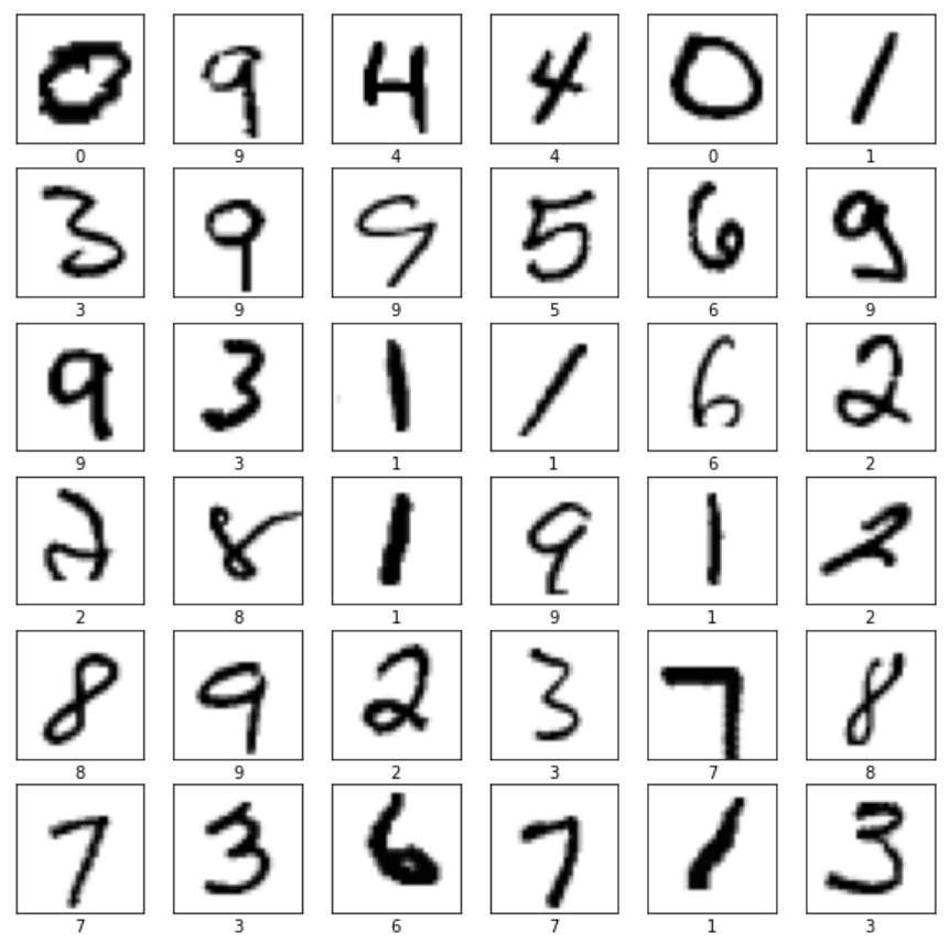
Now let see what there is inside this database by randomly plotting 36 pictures:
In [5]: # set a proper figure dimension
   ...: plt.figure(figsize=(10,10))
   ...:
   ...: # pick 36 random digits in range 0-59999
   ...: # inner bound is inclusive, outer bound exclusive
   ...: random_inds = np.random.choice(60000,36)
   ...:
   ...: for i in range(36):
   ...:     plt.subplot(6,6,i+1)
   ...:     plt.xticks([])
   ...:     plt.yticks([])
   ...:     plt.grid(False)
   ...:     image_ind = random_inds[i]
   ...:     # show images using a binary color map (i.e. Black and White only)
   ...:     plt.imshow(train_images[image_ind], cmap=plt.cm.binary)
   ...:     # set the image label
   ...:     plt.xlabel(train_labels[image_ind])
In all Neural network, we work with floating-point number that has to be in the interval \([0, 1]\). Since our data is in RGB thus assume an integer value between 0 to 255 we perform the following normalization:
In [6]: # from range 0-255 to 0-1
   ...: train_images = (np.expand_dims(train_images, axis=-1)/255.).astype(np.float32)
   ...: train_labels = (train_labels).astype(np.int64)
   ...: test_images = (np.expand_dims(test_images, axis=-1)/255.).astype(np.float32)
   ...: test_labels = (test_labels).astype(np.int64)
1.3.3. Model building
Now we are going to build our basic CNN
First, we open a new section of our Notebook.
# Model building
Then, using the TF (Keras) API we will simply build the VGG16 as follow:
In [7]: def create_model():
   ...:     # Input block
   ...:     input_tensor = layers.Input(shape=[train_images.shape[1], train_images.shape[2], 1],
   ...:                                 name="input")
   ...:     # Block 1
   ...:     x = layers.Conv2D(
   ...:             24, (3, 3), activation='relu', padding='same', name='block1_conv1')(input_tensor)
   ...:     x = layers.MaxPooling2D((2, 2), name='block1_pool')(x)
   ...:     # Block 2
   ...:     x = layers.Conv2D(
   ...:             36, (3, 3), activation='relu', padding='same', name='block2_conv1')(x)
   ...:     x = layers.MaxPooling2D((2, 2), strides=(2, 2), name='block2_pool')(x)
   ...:     # Classification block
   ...:     x = layers.Flatten(name='flatten')(x)
   ...:     x = layers.Dense(128, activation='relu', name='fc1')(x)
   ...:     x = layers.Dropout(rate=0.5)(x)
   ...:     prob = layers.Dense(10, activation="softmax",
   ...:                         name='predictions')(x)
   ...:
   ...:     model = tf.keras.Model(input_tensor, prob)
   ...:     return model
Let us call the function and build the model
In [8]: model = create_model()
And let us see if if is all in order
In [9]: model.summary()
1.3.4. Model compiling
Now we have to “compile” the model. Which means choose the loss fanction, the traingin strategy and optimizer (and learning rate), and the right metrics for the evaulation.
Loss Function: it is the critera by which to evaluate the accuracy of the model. The traing goal is to minimize this function. For this case we choose the Sparse Categorical Crossentropy
Optimizer: It defines the model weights serchin criteria to minimize the loss function. In this tutotrial we choose the common Adam
Metrics: It the wey yo evaulate the goodness of the model. For this kind of model usualy we choose the Accuracy
As usual let us open a new section:
# Model compiling
In [10]: learning_rate=1e-2
   ...: optimizer = tf.keras.optimizers.Adam(learning_rate=learning_rate)
   ...: loss='sparse_categorical_crossentropy'
   ...: metrics=['accuracy']
   ...:
   ...: model.compile(
   ...:     optimizer,
   ...:     loss,
   ...:     metrics,
   ...: )
1.3.5. Training
Since it is impossible to feed all our database in a one-shot, we split it into smaller sub-sets called batch then we train the model multiple times to allow the convergence.
As usual let us open a new section:
# Training
And let us train the model with the train_images dataset.
In [10]: batch_size = 256
   ...: epochs = 10
   ...:
   ...: history = model.fit(
   ...:     train_images,
   ...:     train_labels,
   ...:     batch_size,
   ...:     epochs,
   ...: )
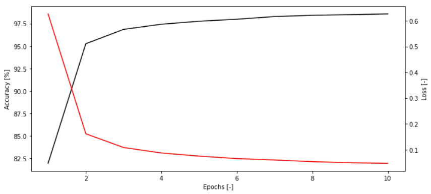
At the end of the training, we can plot the learning curve of the model:
In [11]: # Plot traing loop
   ...: accuracy = np.array(history.history['accuracy'])
   ...: loss = np.array(history.history['loss'])
   ...: epochs_i = np.arange(1,11)
   ...:
   ...: fig = plt.figure(figsize=(10,4.5))
   ...: ax = fig.add_subplot('111')
   ...: ax_twin = ax.twinx()
   ...: ax.plot(epochs_i, accuracy*100, color='k')
   ...: ax_twin.plot(epochs_i, loss, color='r')
   ...: ax.set_xlabel('Epochs [-]')
   ...: ax.set_ylabel('Accuracy [%]')
   ...: ax_twin.set_ylabel('Loss [-]')
   ...: plt.tight_layout()
   ...: plt.show()
1.3.6. Results
We can now visulize the result.
As usual let us open a new section:
# Results
Then we have to collect the prediction for the Test set test_images
In [12]: predictions = model.predict(test_images)
We write some function useful to visualizing the data:
# Define classnames for improved readability
class_names = ['Zero', 'One', 'Two', 'Three', 'Four',
            'Five', 'Six', 'Seven', 'Eight', 'Nine']

def plot_image(i, predictions_array, true_label, img):
    predictions_array, true_label, img = predictions_array, true_label[i], img[i]
    plt.grid(False)
    plt.xticks([])
    plt.yticks([])

    plt.imshow(img, cmap=plt.cm.binary)

    predicted_label = np.argmax(predictions_array)
    if predicted_label == true_label:
        color = 'blue'
    else:
        color = 'red'

    plt.xlabel("{} {:2.0f}% ({})".format(class_names[predicted_label],
                                    100*np.max(predictions_array),
                                    class_names[true_label]),
                                    color=color)

def plot_value_array(i, predictions_array, true_label):
    predictions_array, true_label = predictions_array, true_label[i]
    plt.grid(False)
    plt.xticks(range(10))
    plt.yticks([])
    thisplot = plt.bar(range(10), predictions_array, color="#777777")
    plt.ylim([0, 1])
    predicted_label = np.argmax(predictions_array)

    thisplot[predicted_label].set_color('red')
    thisplot[true_label].set_color('blue')
And let us see the prediction versus the ground truth:
In [13]: num_rows = 5
   ...: num_cols = 3
   ...: num_images = num_rows*num_cols
   ...: plt.figure(figsize=(2*2*num_cols, 2*num_rows))
   ...: for i in range(num_images):
   ...:     plt.subplot(num_rows, 2*num_cols, 2*i+1)
   ...:     plot_image(i, predictions[i], test_labels, np.squeeze(test_images))
   ...:     plt.subplot(num_rows, 2*num_cols, 2*i+2)
   ...:     plot_value_array(i, predictions[i], test_labels)
   ...: plt.tight_layout()
   ...: plt.show()
1.4. Excercise
Following the same steps, build a similar CNN for the Fashion MNIST database https://github.com/zalandoresearch/fashion-mnist. First test if all is working by only changing the Data collection and preprocessing command with:
In [3]: mnist = tf.keras.datasets.fashion_mnist
   ...: (train_images, train_labels), (test_images, test_labels) = mnist.load_data()
Then, one at the time, add the following features at your code:
Build a custom data pipeline (see guide Tensorflow Data) to load the Fashion MNIST.
Add an additional convolutional block with 48 3x3 kernels to the model.
Write the training loop from scratch (see guide Tensorflow Training loop).
Add to the model callback option to save checkpoint every 10 epochs (see guide Tensorflow Checkpoint).
Save the model (see guide Tensorflow Save model).
For help with all these tasks, consult the Tensorflow Guide, and the internet is full of answers to your question.